Emiliano Rossi ID
Médico cardiólogo. Departamento de Investigación. Hospital Italiano de Buenos Aires.
Ciudad Autónoma de Buenos Aires, Argentina.
Acta Gastroenterol Latinoam 2022;52(1):7-10
Recibido: 19/01/2022 / Aceptado: 18/03/2022 / Publicado en www.actagastro.org el 30/03/2022 / https://doi.org/10.52787/agl.v52i1.164

¿Qué es el análisis de sobrevida?
En un gran número de situaciones clínicas, no solo nos interesa estudiar si se presenta o no un evento, sino también determinar en qué momento del seguimiento se produce.
El análisis de sobrevida es un conjunto de procedimientos estadísticos para el análisis de datos en los cuales la variable de resultado es el tiempo hasta que un evento ocurre.
¿Para qué se utiliza?
Las primeras aplicaciones de este análisis estudiaron el tiempo desde el inicio de un tratamiento hasta la muerte, de ahí el nombre de sobrevida. Posteriormente, su aplicación se extendió a otras situaciones de interés clínico (tiempo a la reinternación, al abandono del tratamiento, al retorno laboral luego de una cirugía, etc.), por lo que una denominación más adecuada es la de análisis de tiempo al evento.
Los objetivos del análisis de sobrevida son: a) estimar e interpretar la sobrevida, b) comparar la sobrevida entre distintos grupos y c) evaluar la relación de distintas variables explicativas con la sobrevida.1
¿Cuál es el punto final evaluado?
Habitualmente, se estudia un solo evento de interés, aunque puede establecerse un punto final combinado (considerándose para el análisis el primer componente que se presente). En otras situaciones de mayor complejidad, se consideran eventos recurrentes o competitivos.1
¿En qué diseños de estudios se aplica?
Los diseños donde puede verse aplicada la metodología del análisis de sobrevida son los estudios de cohortes y los ensayos clínicos.
¿Qué información se necesita registrar para su implementación?
Para poder aplicar este análisis, se necesita determinar, al inicio del estudio, qué pacientes son susceptibles de sufrir el evento, excluyendo a aquellos que no lo son, y luego registrar la fecha en la que ocurre el evento de interés o la fecha de finalización del seguimiento en los casos en los que no se hubiera presentado.
¿Qué es la función de sobrevida y la función de riesgo?
Son dos conceptos íntimamente relacionados. La función de sobrevida S (t) es definida como la probabilidad de sobrevivir hasta un determinado tiempo. La función de riesgo h (T) es la probabilidad condicional de presentar el evento a determinado tiempo, dado que el individuo ha sobrevivido hasta ese momento.2 El gráfico de la función de sobrevida es la curva de sobrevida.
¿Qué es la censura?
Es un concepto relevante a tener en cuenta al realizar un análisis de sobrevida. El tiempo hasta la ocurrencia del evento no es visible en todos los pacientes, está censurado porque el seguimiento se ha interrumpido (por ej. debido a pérdida de seguimiento del paciente): no hay forma de saber cuándo ocurrirá el evento a partir de ese momento. Las situaciones en las que puede haber tiempo de sobrevida censurado ocurren cuando hay pérdida de seguimiento, se produce un retiro del estudio o este finaliza y el paciente todavía no ha presentado el evento.1
¿Cuál es la ventaja de aplicar este análisis?
La ventaja de utilizar el análisis de sobrevida es que nos permite considerar la información disponible de todos los pacientes, no solo de los que llegaron al final del seguimiento. Cada paciente aporta información durante el periodo en el que permane en el estudio, aunque luego se pierda el seguimiento. Los pacientes que presentan censura temprana contribuyen con menos información que quienes son seguidos por un largo tiempo. Todas las observaciones aportan alguna información. En cambio, si se incluyera en el análisis solo a los pacientes que finalizaron el estudio, se estaría introduciendo un sesgo.
¿Cuáles son los métodos estadísticos utilizados?
Los métodos más conocidos que permiten manejar la censura, en un análisis de sobrevida, son las curvas de Kaplan-Meier y el modelo de riesgos proporcionales de Cox.
Las curvas de Kaplan-Meier grafican la proporción de pacientes que han sobrevivido en el tiempo en cada grupo de tratamiento (exposición). La altura de la curva de Kaplan-Meier, al final de cada intervalo de tiempo, se determina tomando la proporción de pacientes que permanecieron sin el evento al final del intervalo anterior y multiplicándola por la proporción de pacientes que sobrevivieron al final del intervalo actual. Este proceso iterativo de multiplicación de probabilidades comienza en el primer intervalo temporal y continúa hasta el último. La curva de sobrevida no se modifica al momento en el que una observación es censurada, pero en el periodo siguiente se excluye del número de personas en riesgo a las que han presentado censura.
La comparación de las curvas de Kaplan-Meier se lleva a cabo mediante el log-rank test.2 Esta prueba testea la hipótesis nula de que no hay diferencia entre las curvas de sobrevida de los distintos grupos y para ello considera los eventos observados y los esperados para cada grupo.
El modelo de riesgos proporcionales de Cox permite resolver el problema de la censura y, además, ajustar por covariables (por ej. confundidores). La medida de resumen del modelo es el hazard ratio (HR). El HR es la relación entre el riesgo (hazard) del grupo de interés y el de referencia. Nos permite estimar cuánto aumenta el riesgo de sufrir el evento por cada unidad de aumento de la variable explicativa. Por ejemplo, si el HR es 1,25 para la edad (en años), esto significa que por cada aumento de un año el individuo tiene un 25% más de riesgo de presentar el evento de interés.
¿Cuáles son las limitaciones del modelo de riesgos proporcionales de Cox?
Este modelo requiere que se cumplan dos supuestos.3 El primero es que los datos censurados sean independientes del resultado de interés. Esto no se cumple en el caso de pacientes que, por haber presentado el evento de interés, pierden el seguimiento. El segundo supuesto es que los riesgos sean proporcionales, es decir, que el HR sea constante durante toda la duración del estudio. Esto significa que si aumenta (o disminuye) el riesgo en el grupo expuesto, en forma concomitante debe aumentar (o disminuir) en el grupo comparador, manteniéndose constante la relación entre ambos. Si estos supuestos no se cumplen, los resultados del modelo no son válidos.
¿Cuándo no se cumple el supuesto de proporcionalidad de los hazards?
El HR no es constante cuando los efectos del tratamiento cambian en el tiempo o cuando la susceptibilidad de sufrir el evento varía entre los individuos de uno de los grupos (dándose el fenómeno de agotamiento de susceptibles).4 Estas situaciones son frecuentes en los estudios clínicos y se debe tener en cuenta que, aunque se apliquen test para evaluar la proporcionalidad de los hazards, estos pueden no tener suficiente poder.4, 5
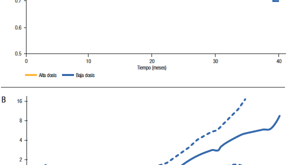
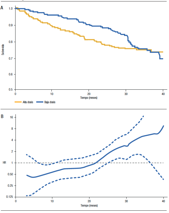
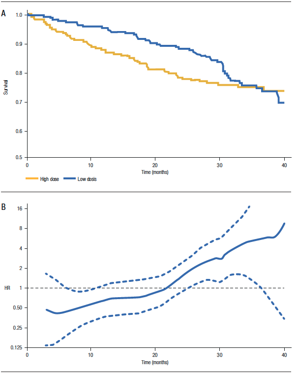
A los fines prácticos, debemos sospechar que el supuesto de proporcionalidad de los hazards no se cumple cuando las curvas de sobrevida presentan cambios manifiestos en sus pendientes. En la Figura 1A, que muestra la sobrevida de dos grupos de pacientes con mieloma múltiple tratados con bajas y altas dosis de dexametasona (ECOG Study), se observa que, en el periodo inicial, las curvas de sobrevida son divergentes. Luego tienden a ser paralelas y finalmente, convergen (llegando incluso a entrecruzarse). Si observamos el gráfico del HR a lo largo del seguimiento (Figura 1B), notamos que el HR no es constante. Inicialmente, es menor a 1 (lo que indica que el hazard del grupo baja dosis es menor), posteriormente hacia la mitad del seguimiento es igual a 1 y finalmente, es mayor a 1. El HR estimado, en este estudio, fue de 0,87, lo que no debe interpretarse como una reducción uniforme del 13% de la mortalidad para el grupo baja dosis.5
¿Qué hacer si se viola la asunción de proporcionalidad de los hazards?
En estos casos, no debemos utilizar el HR sino otras medidas para comparar las diferencias de sobrevida entre los grupos. Una de las alternativas que disponemos es la razón de tiempo de sobrevida media restringido. El tiempo de sobrevida media restringido (RMST, según sus siglas en inglés) representa el promedio grupal de tiempo libre de eventos durante el periodo. Se calcula estimando el área bajo la curva de Kaplan-Meier hasta un tiempo determinado. En el estudio mencionado (ECOG), el RMST a 40 meses del grupo baja dosis tiene un área bajo la curva igual a 35,1 meses (lo que significa que se espera que un paciente de este grupo viva 35,1 meses de los 40 meses de seguimiento). En cambio, en el grupo alta dosis, el área bajo la curva representa 33,3 meses; siendo entonces la razón de RMST = 35,1/40 = 1,06 (IC 95% 1,00 -1,13).5
Figura 1. A) Curvas de sobrevida según tratamiento, B) Estimación del HR (y su IC 95%) durante el seguimiento.
Aviso de derechos de autor
 © 2022 Acta Gastroenterológica Latinoamericana. Este es un artículo de acceso abierto publicado bajo los términos de la Licencia Creative Commons Attribution (CC BY-NC-SA 4.0), la cual permite el uso, la distribución y la reproducción de forma no comercial, siempre que se cite al autor y la fuente original.
Cite este artículo como: Rossi E. Introducción al análisis de sobrevida. Acta Gastroenterol Latinoam. 2022;52(1):7-10 https://doi.org/10.52787/agl.v52i1.164
Referencias
- Kleinbaum DG, Klein M. Survival Analysis: A Self-Learning Text. New York: Springer; 2012.
- Bewick V, Cheek L, Ball J. Statistics review 12: Survival analysis. Critical Care 2004;8:389-395.
- Tolles J, Lewis RJ. Time-to-Event Analysis. JAMA 2016;315 (10):1046-1047.
- Stensrud MJ, Hernán MA. Why Test for Proportional Hazards?. JAMA 2020;323(14):1401-1402.
- Uno H, Claggett B, Tian L, et al. Moving Beyond the Hazard Ratio in Quantifying the Between-Group Difference in Survival Analysis. J Clin Oncol 2014;32:2380-2385.
Correspondencia: Emiliano Rossi
Correo electrónico: emiliano.rossi@hospitalitaliano.org.ar
Acta Gastroenterol Latinoam 2022;52(1):7-10
Introduction to Survival Analysis
Emiliano Rossi ID
Cardiologist. Department of Investigation. Hospital Italiano de Buenos Aires.
City of Buenos Aires, Argentina.
Acta Gastroenterol Latinoam 2022;52(1):11-14
Received: 19/01/2022 / Accepted: 18/03/2022 / Published online: 30/03/2022 / https://doi.org/10.52787/agl.v52i1.164
What is Survival Analysis?
In many clinical situations, we are interested not only in studying whether an event occurs, but also in determining at what point it take place during the follow-up.
Survival analysis is a set of statistical procedures for data analysis in which the outcome variable is the time until an event occurs.
What Is It for?
The first applications of this analysis studied the time from the start of treatment to death, hence the name “survival”. Subsequently, it was extended to other situations of clinical interest (time to readmission, treatment abandonment, return to work after surgery, etc.), so that a more appropriate name is time-to-event analysis.
The objectives of survival analysis are: a) to estimate and interpret survival, b) to compare survival between different groups, and c) to evaluate the relationship of different explanatory variables with survival.1
What Is the Endpoint Evaluated?
Usually a single event of interest is studied, although a combined endpoint may be established (the first component to be considered for the analysis). In other more complex situations, recurrent or competitive events are considered.1
In What Study Designs Is Applied?
The designs where the survival analysis methodology can be applied are cohort studies and clinical trials.
What Information Needs to Be Recorded for Its Implementation?
To apply this analysis, it is necessary to determine at the beginning of the study which patients are susceptible to the event, excluding those who are not. Then record the date on which the event of interest occurs or the end date of follow-up, in the cases where the event did not occur.
What Is the Survival Function and the Hazard Function?
They are two closely related concepts. The survival function S (t) is defined as the probability of surviving at a given time. The hazard function h (T) is the conditional probability of the event occurring at a certain time, given that the individual has survived to that time.2 The graph of the survival function is the survival curve.
What Is Censorship?
It is a relevant concept to consider when performing a survival analysis. The time to the occurrence of the event is not visible in all patients, it is censored because follow-up has been interrupted (i.e., the patient has been lost to follow-up). There is no way of knowing when the event will occur thereafter. The situations in which survival time can be censored are: when there is loss to follow-up, when there is withdrawal from the study, and when the study ends and the patient has not yet presented the event.1
What Is the Advantage of Applying this Analysis?
The advantage of using the survival analysis is that it allows us to consider the information available on all patients, not just those who reached the end of the follow-up. Each patient provides information during the period they were in the study, even if they later lost follow-up. Thus, patients who present early censoring provide less information than those who are followed for a long time. Therefore, all observations contribute some information. On the other hand, if only patients who completed the study were included in the analysis, a bias would be introduced.
What Are the Statistical Methods Used?
The best-known methods that allow handling censorship in survival analysis are the Kaplan-Meier curves and the Cox proportional hazards model.
Kaplan-Meier curves plot the proportion of patients who have survived over time in each treatment (exposure) group. The height of the Kaplan-Meier curve at the end of each time interval is determined, by taking the proportion of patients who were event-free at the end of the previous interval and multiplying it by the proportion of patients who survived at the end of the current interval. This iterative process of multiplying probabilities begins at the first-time interval and continues to the last. The survival curve is not modified when an observation is censored, but, in the following period, those who have been censored are excluded from the number of people at risk.
Comparison of the Kaplan-Meier curves is carried out using the log-rank test.2 This test examines the null hypothesis that there is no difference between the survival curves of the different groups, considering the observed events for each group.
The Cox proportional hazards model allows solving the censoring problem and, in addition, adjusting for covariates (e.g., confounders). The summary measure of the model is the hazard ratio (HR). The HR is the ratio between the hazard (risk) of the group of interest and the reference group. It allows us to estimate how much the risk of suffering the event increases for each unit increase in the explanatory variable. For example, if the HR is 1.25 for age (in years), this means that for each increase in one year the individual has a 25% higher risk of presenting the event of interest.
What Are the Limitations of the Cox Proportional Hazards Model?
This model requires two assumptions to be met.3 The first is that the censored data must be independent of the outcome of interest. This is not true in the case of patients who are lost to follow-up, because of the event of interest. The second assumption is that the hazards are proportional, meaning that the HR is constant throughout the duration of the study. This means that, if the risk increases (or decreases) in the exposed group, it should concomitantly increase (or decrease) in the comparator group, keeping the relationship between the two-remaining constant. If these assumptions are not met, the model results are not valid.
When Is the Hazard Proportionality Assumption not Met?
The HR is not constant when the effects of the treatment change over time or when the susceptibility to suffer the event varies among individuals in one of the groups (giving rise to the phenomenon of exhaustion of susceptibles).4 These situations are frequent in clinical studies. It must be taken into account that, even if tests are applied to evaluate the proportionality of the hazards, they may not have sufficient power.4, 5
For practical purposes, we should suspect that the hazard proportionality assumption is not fulfilled when the survival curves show obvious changes in their slopes. Figure 1A shows the survival of two groups of patients with multiple myeloma treated with low and high doses of dexamethasone (ECOG Study): in the initial period, the survival curves are divergent, then they tend to be parallel and finally, converge (even intersecting). If we observe the HR graph throughout the follow-up (Figure 1B), we notice that the HR is not constant. Initially, it is less than 1 (indicating that the hazard of the low-dose group is lower), then towards the middle of follow-up it is equal to 1 and finally, it is greater than 1. The estimated HR in this study was 0.87, which should not be interpreted as a uniform 13% reduction in mortality for the low-dose group.5
What to Do If the Hazard Proportionality Assumption Is Violated?
In these cases, we should not use HR but rather other measures to compare the differences in survival between groups. One of the alternatives available is the restricted median survival time ratio. The restricted median survival time (RMST) represents the group average of event-free time during the period. It is calculated by estimating the area under the Kaplan-Meier curve up to a given time. In the aforementioned study (ECOG), the RMST at 40 months of the low-dose group has an area under the curve equal to 35.1 months (meaning that a patient in this group is expected to live 35.1 months out of 40 months of follow-up). In contrast, in the high-dose group, the area under the curve represents 33.3 months. Thus, the ratio of RMST = 35.1/40 = 1.06 (95% CI 1.00-1.13).5
Figure 1. A) Survival curves according to treatment, B) HR estimate (and 95% CI) during follow-up.
Copyright© 2022 Acta Gastroenterológica latinoamericana. This is an open-access article released under the terms of the Creative Commons Attribution (CC BY-NC-SA 4.0) license, which allows non-commercial use, distribution, and reproduction, provided the original author and source are acknowledged.
Cite this article as: Rossi E. Introduction to Survival Analysis. Acta Gastroenterol Latinoam. 2022;52(1):11-14. https://doi.org/10.52787/agl.v52i1.164
References
- Kleinbaum DG, Klein M. Survival Analysis: A Self-Learning Text. New York: Springer; 2012.
- Bewick V, Cheek L, Ball J. Statistics review 12: Survival analysis. Critical Care 2004;8:389-395.
- Tolles J, Lewis RJ. Time-to-Event Analysis. JAMA 2016; 315(10): 1046-1047.
- Stensrud MJ, Hernán MA. Why Test for Proportional Hazards?. JAMA 2020;323(14):1401-1402.
- Uno H, Claggett B, Tian L, et al. Moving Beyond the Hazard Ratio in Quantifying the Between-Group Difference in Survival Analysis. J Clin Oncol 2014;32:2380-2385.
Correspondence: Emiliano Rossi
Email: emiliano.rossi@hospitalitaliano.org.ar
Acta Gastroenterol Latinoam 2022;52(1):11-14